

I am just coming out of a period of intense reading and writing for my end-of-first-year qualifying proposal in my PhD program at NYU. I’m not quite done, as I still need to defend it in a couple of weeks. In the meantime, I need a little break from thinking about it. Hence, this post (where I am doing more writing, yes, but it is not related to my qualifying exam!).
Like for most people, news on the COVID-19 pandemic has dominated my social media feeds, as well as my conversations with people over the last month. I keep seeing these projection models, and it makes me think of an infectious disease modeling course I took (taught by Derek Cummings and Justin Lessler) during my Master’s a few years ago, which taught us how to build simple models for infectious disease transmission and control. So, I dug up some old notes to see if I could relearn some of that, and now in this tutorial, I will describe how to use a simple model to explore two questions.
1) In a completely susceptible population, how soon would SARS-CoV2 infections peak, and how would social distancing affect the peak of the epidemic curve?
2) What percentage of individuals would need to be vaccinated for there to be sufficient herd immunity to protect the whole population or prevent an epidemic?
All of the code is to be run on R. Download RStudio here.
A caveat here, and I can’t stress this enough, is that the model I will use is probably the simplest possible one, and is by no means the best model to use to model the transmission of any virus, let alone SARS-CoV2 transmission. Think of this as a science communication exercise, where you gain a basic sense of how models work, and how measures like social distancing help.
First, some theoretical background. The basic model we will use is a mass-action SIR (Susceptible, Infectious, Recovered) model, a simple kind of compartment model. It assumes random mixing of individuals in a population, and individuals can belong to one of three categories or compartments (Susceptible, Infectious, Recovered) and move between between them.
In our model, susceptible individuals become infected by infectious individuals, and infected individuals recover at a certain rate. Recovered individuals are considered resistant or immune, and cannot be infected again. Thus, there are three important rates of change for us to consider: dS/dt, the rate of change of susceptible individuals, dI/dt, the rate of change of infectious individuals, and dR/dt, the rate of change of recovered individuals.
What do these rates of change depend on? Let’s visualize them as compartments, where individuals can move between susceptible, infectious, and recovered compartments.

dS/dt, or the rate of change of susceptible individuals, is basically the rate at which susceptible individuals become infected (and hence infectious). It depends linearly on the number of susceptible individuals (S), the number of infectious individuals, (I), and the rate or probability of infectious contact between two individuals, (β). dS/dt will be a negative rate as the number of susceptible individuals can only decrease as individuals become infected.

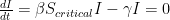
dI/dt, or the rate of change of infectious individuals, depends on the rate at which susceptible individuals become infected and the rate at which infected individuals recover. The latter depends linearly on the number of infected individuals (I), and the recovery rate of individuals, (γ), and is negative because recovery results in a decrease in the number of infected individuals.

Finally, dR/dt, or the rate of change of recovered individuals, is the rate at which infected individuals recover. This time, this is positive, as this rate contributes to an increase in the number of recovered individuals.

β and γ represent constants. When we solve these ordinary differential equations with the starting values of S and I, we get new values of S and I. We then solve the equations with these new values, and keep doing this to see how the numbers of susceptible, infectious, and recovered individuals change over time. Don’t worry, this whole process will be automated.
Now, starting values of S and I are simple to define in our model, as they just represent the starting numbers of susceptible and infectious individuals. But how do we obtain β and γ?
γ is simply the inverse of the duration of infectiousness. If infected individuals remain infectious for two days, the rate of recovery is ½ per day. To get β, let’s for our purposes understand it in terms of its relationship with a variable called R0 in a mass-action model (this formula can change, based on the kind of model we use).

R0, or the basic reproduction number, refers to the number of individuals each infectious individual will infect in a completely susceptible population. For reference, influenza has an R0 of around 2-3, while measles has an R0 of 12-18 (a nightmare without vaccines). An R0 of less than zero means the pathogen will be self-limiting as each individual on average would be passing it on to less than one individual. N is the total number of individuals.
Now, let’s define our constants. While the number may vary considerably, let’s take the reasonable estimate based on current evidence that the duration of infectiousness is ~10 days. We will run our simulations on a population of 1,000 individuals, starting with one infectious individual. R0 has been estimated to be somewhere between 1.5 and 3.5, so let us define it as 2.5. We will use R0, γ, and the total number of individuals to estimate β. We will run our simulations over 365 days.
Now, open up RStudio. When defining functions (like x <- function(){…}), you have to run all of the lines together. The same applies to if statements and lines connected by +. The best way to do it would be to open a new R script, copy-paste all of the code into it, and run them from there. You could also copy-paste the code from each box into the console one by one directly.
First, install a package for solving differential equations, and load it:
# These hashes indicate comments, and not actual code
# Command for installing packages if they are not already installed
if (!require('deSolve')) {
  install.packages("deSolve")
}
# Command for loading a package
library(deSolve)
Define the constants and initial values:
R <- 2.5
duration <- 10
Gamma<- 1/duration

# Initial values of S, I, and R individuals
i.S <- 999
i.I  <- 1
i.R <- 0

# Compute beta from R, gamma, and total number of indviduals
Beta<- (R * Gamma)/(i.S + i.I + i.R)
Time <- 365
On R, there are many built-in functions.
# Create a vector of numbers
numbers <- c(1,2,3,4,5,6)

# Get highest number
max(numbers)
## [1] 6
# Get mean
mean(numbers)
## [1] 3.5
# Get standard deviation
sd(numbers)
## [1] 1.870829
# Learn about the arguments contained with a function
# by running commands like the following without the hash
# ?sd
You get the idea. We need a function to run our SIR model, but R doesn’t have a built-in function for it. We’ll have to write our own:
runSIR <- function(beta=Beta,
                   gamma=Gamma,
                   initial.state= c(S=i.S, I=i.I, R=i.R),
                   max.time = Time) {

  # Within the function, beta, gamma etc. represent arguments or inputs
  # We have set the default inputs as the constants and
  # initial values we defined above

  # The seq function creates intervals of 1 between 0 and the inputted max.time
  times <- seq(0,max.time,1)

  # beta and gamma will remain constant
  # These are the parameters in our ordinary differential equations (ODEs)
  parameters <- c(beta=beta,gamma=gamma)

  # This runs the ODE-Solver from the deSolve package
  # The arguments are: the state of the system (y), the time steps,
  # a function for the actual differential equations, and the parameters
  sir.output <- lsoda(initial.state, times, dx.dt, parameters)
  # y is initially the initial.state, but when the function is run, this value
  # will be updated at every step, as the values of S, I, and R get updated

  # Notice that the differential equations function (dx.dt) has not been set yet,
  # that will be done in the next function

  # Finally, we will return the output as a dataframe
  return(as.data.frame(sir.output))
}
Next, we write up a function to calculate for each time step (for instance, from day 1 to day 2) the changes in S, I, and R.
dx.dt <- function(t, y, parameters) {
  # The arguments are:
  # t is the current time
  # y is the current state (that is, the values of S, I, and R at the current step)
  # parameters contains beta and gamma, as defined above

  # Equation to calculate the change in susceptibles
  # (The square brackets are for subsetting out the relevant information from the vectors
  # parameters contains both beta and gamma, and in this step, we are extracting the beta variable
  # Similarly, y contains S, I, and R, and we extract them as they are needed
  # The equations should be familiar to you from above)
  dS <- - parameters["beta"] * y["S"] * y["I"]

  # Equation to calculate the change in infectious individuals
  dI <- parameters["beta"] * y["S"] * y["I"] - parameters["gamma"] * y["I"]

  # Equation to calculate the change in recovered individuals
  dR <- parameters["gamma"] * y["I"]

  # Return the results
  return(list(c(dS, dI, dR)))
}
The output of runSIR will be a dataframe with 365 rows (one for each time step) and four columns (“time”, “S”, “I”, and “R”). While that’s nice, we want to be able to plot them. Let’s write a simple plotting function.
# My function uses functions from a package called ggplot2,
# which is great for making publication quality figures on R.
# I could also have used base R plotting functions, but
# ggplot2 is much more easily customizable

plot.ode <- function(lsoda.output)  {

  # The sole argument here is the output generated by
  # the runSIR function, which used the lsoda function
  # from the deSolve package

  # Load two packages we will need
  library(reshape2)
  library(ggplot2)

  # For easier plotting with ggplot, manipulate the dataframe so that
  # the S, I, and R values all come into a single column
  lsoda.melted <- melt(lsoda.output,id.vars = "time")

  # Change default column names
  colnames(lsoda.melted) <- c("Time","Compartment","Individuals")

  # We will plot proportions rather than numbers of individuals
  lsoda.melted$Individuals <- lsoda.melted$Individuals / (i.S + i.I + i.R)

  # Plot the dataframe while setting axis labels and line colors
  ggplot(data = lsoda.melted, mapping = aes(y = Individuals, x = Time, color = Compartment))+
    geom_line()+
    xlab("Time (Days")+
    ylab("Proportion of Individuals")+
    scale_color_manual(values=c("blue","red","green"))
}
Once we run the above three sections of code, these functions become available to us in R’s global environment. We can then run our SIR model and plot it.
# Run the SIR model while storing it as SIR.output
# We don't actually need to put in any arguments as
# we already defined the default variables in the beginning
SIR.output <- runSIR()

# Take a look at the first few rows
head(SIR.output)
##   time        S        I         R
## 1    0 999.0000 1.000000 0.0000000
## 2    1 998.7306 1.161506 0.1078745
## 3    2 998.4178 1.348999 0.2331675
## 4    3 998.0547 1.566623 0.3786783
## 5    4 997.6332 1.819178 0.5476556
## 6    5 997.1439 2.112208 0.7438627
# Plot it
plot.ode(SIR.output)

So far so good! Now, how would this look if social distancing measures were put in place? Social distancing should reduce the rate or probability of infectious contacts between individuals. This should affect dS/dt and dI/dt through affecting β.
Let’s assume that a particular social distancing measure like closing schools reduces the rate of infectious contacts by 30%. We can modify our β by multiplying it by 0.7. Let’s see how different the plot looks.
# Run our runSIR function, but this time, modify beta
sdist.output <- runSIR(beta = 0.7 * Beta)

plot.ode(sdist.output)

Let’s plot just the number of infectious individuals from the two models for a simpler visual comparison of the epidemic peaks.
# We are going to combine our outputs, but before that,
# let's add a column called "Strategy" so that they
# can be differentiated after merging
SIR.output$Strategy <- "No social distancing"

sdist.output$Strategy <- "Social distancing"
# Combine our dataframes
combined <- rbind(SIR.output,sdist.output)

# Convert the numbers into proportions
# We will only plot I, but doing it for S and R
# for consistency
combined$S <- combined$S / (i.S + i.I + i.R)
combined$I <- combined$I / (i.S + i.I + i.R)
combined$R <- combined$R / (i.S + i.I + i.R)

library(ggplot2)
ggplot(data = combined, mapping = aes(x = time, y = I, linetype = Strategy))+
  geom_line(color = "red")+
  xlab("Time (Days)")+
  ylab("Proportion of population infected")+
  scale_linetype_manual(values = c("solid","dashed"))

In our model, social distancing not only reduces the total number of infected cases (compare the recovered proportions with and without social distancing), but more significantly, also flattens the peak of the epidemic curve, which means that fewer individuals are infected (and hence may need healthcare) at any time point, thereby reducing the burden on the healthcare system.
We’ve answered the first of our two questions. You can play around with the model. Note that no one dies in this model. Could you add a compartment for deceased individuals and define a death rate? People who do this professionally play around with many more complex variables such as density, geography, migration, and age-dependence, and define constants in more sophisticated ways. Note also that our model is deterministic, in that if you run it again, it will produce the same output. Stochastic models incorporate chance, and are hence perhaps more realistic. Finally, data from real outbreaks are also often fit to such models to infer parameters like R0.
For our second question, we don’t actually need any fancy coding, just some math. In a mass-action SIR model, it is possible to identify a critical threshold of the proportion of susceptible individuals, above which cases would grow in number and below which cases would decline. At this threshold, dI/dt should be zero; if it drops below zero, infected individuals will decline, and if it rises above zero, infected individuals will increase. We can solve this equation to compute the critical threshold of susceptibles. The critical vaccination threshold, V, is 1 minus this number, and represents the proportion of individuals that must be protected or non-susceptible for dI/dt to be zero.


Recall our earlier equation for R0. Since we are thinking in terms of proportions here, the total number is 1, so we can rewrite that equation as:

V can thus be directly calculated in our model directly from R0:

What is V for our pathogen?
# We can't directly use the beta we calculated above
# because that was scaled by the total number of individuals
# Here we recalculate beta for a "population" of 1,
# from which we can generate proportions
Beta_raw <- R * Gamma

# Calculate V
V = 1 - (Gamma/Beta_raw)
V
## [1] 0.6
You would get the same value with the other formula for V.
The interpretation here would be that 60% of the population would need to be vaccinated to ensure protection for the whole population. You can see this in action in our model by adjusting the initial S, I, and R values to have 60% individuals in the R compartment (which, in this case, just represents immune individuals). The number of infected individuals can never rise if 60% of the individuals are protected to begin with, so infections will die out.
